Crawling Data by Using Scrapy
Blog Post: Image Classification
In this blog post, I will use several skills and concepts related to image classification in Tensorflow.
Tensorflow Datasets provide a convenient way for us to organize operations on our training, validation, and test data sets. Data augmentation allows us to create expanded versions of our data sets that allow models to learn patterns more robustly. Transfer learning allows us to use pre-trained models for new tasks. Working on the coding portion of the Blog Post in Google Colab is strongly recommended. When training our models, enabling a GPU runtime (under Runtime -> Change Runtime Type) is likely to lead to significant speed benefits.
The Goal
I will teach a machine learning algorithm to distinguish between pictures of dogs and pictures of cats
According to this helpful diagram below, one way to do this is to attend to the visible emotional range of the pet:
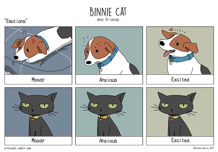
Unfortunately, using this method requires that we have access to multiple images of the same individual. We will consider a setting in which we have only one image for pet. Later I will use tensflow to reliably distinguish between cats and dogs in this case.
Helpful link:
Transfer Learning Tutorial
1. Load Packages and Obtain Data.
We’ll hold our import statements by making a code block and update it when we want to import more statements:
import os
import tensorflow as tf
from tensorflow.keras import datasets, layers, models
from tensorflow.keras import utils
import matplotlib.pyplot as plt
import numpy as np
A sample data set provided by the TensorFlow team that contains labeled images of cats and dogs:
# location of data
_URL = 'https://storage.googleapis.com/mledu-datasets/cats_and_dogs_filtered.zip'

# download the data and extract it
path_to_zip = utils.get_file('cats_and_dogs.zip', origin=_URL, extract=True)

# construct paths
PATH = os.path.join(os.path.dirname(path_to_zip), 'cats_and_dogs_filtered')

train_dir = os.path.join(PATH, 'train')
validation_dir = os.path.join(PATH, 'validation')

# parameters for datasets
BATCH_SIZE = 32
IMG_SIZE = (160, 160)

# construct train and validation datasets
train_dataset = utils.image_dataset_from_directory(train_dir,
                                                   shuffle=True,
                                                   batch_size=BATCH_SIZE,
                                                   image_size=IMG_SIZE)

validation_dataset = utils.image_dataset_from_directory(validation_dir,
                                                        shuffle=True,
                                                        batch_size=BATCH_SIZE,
                                                        image_size=IMG_SIZE)

# construct the test dataset by taking every 5th observation out of the validation dataset
# As the original dataset doesn't contain a test set, we will create one.
# To do so, determine how many batches of data are available in the validation set using tf.data.experimental.cardinality, then move 20% of them to a test set.
val_batches = tf.data.experimental.cardinality(validation_dataset)
test_dataset = validation_dataset.take(val_batches // 5)
validation_dataset = validation_dataset.skip(val_batches // 5)

print('Number of validation batches: %d' % tf.data.experimental.cardinality(validation_dataset))
print('Number of test batches: %d' % tf.data.experimental.cardinality(test_dataset))
Found 2000 files belonging to 2 classes.
Found 1000 files belonging to 2 classes.
Number of validation batches: 26
Number of test batches: 6
By running above code, we have created TensorFlow Datasets for training, validation, and testing. We can think of a Dataset as a pipeline that feeds data to a machine learning model. We use data sets in cases in which it’s not necessarily practical to load all the data into memory.
In our case, we’ve used a special-purpose keras utility called image_dataset_from_directory to construct a Dataset. The most important argument is the first one, which says where the images are located. The shuffle argument says that, when retrieving data from this directory, the order should be randomized. The batch_size determines how many data points are gathered from the directory at once. Here, for example, each time we request some data we will get 32 images from each of the data sets. Finally, the image_size specifies the size of the input images, just like you’d expect.
Working with Datasets
We can get a piece of a data set using the take method; e.g. train_dataset.take(1) will retrieve one batch (32 images with labels) from the training data.
Let’s briefly explore our data set. Write a function to create a two-row visualization. In the first row, show three random pictures of cats. In the second row, show three random pictures of dogs. We can see some related code in the linked tutorial above, although we’ll need to make some modifications in order to separate cats and dogs by rows. A docstring is not required.
def print_cats_and_dogs(train_dataset):
    class_names = train_dataset.class_names

    cat, dog, index = 0, 0, 0
    fig,ax = plt.subplots(2, 3, figsize=(10, 10))
    for images, labels in train_dataset.take(1):
      for i in range (100):
        if (class_names[labels[i]] == 'cats'):
          if (cat >= 3):
            continue
          index = cat + 0
          cat += 1
        else:
          if (dog >= 3):
            continue
          index = dog + 3
          dog += 1

        ax.flat[index].imshow(images[i].numpy().astype("uint8"))
        ax.flat[index].set(title=class_names[labels[i]])
        ax.flat[index].axis("off")

        if (index == 5): # when we have 6 images, break the loop
          break


print_cats_and_dogs(train_dataset)
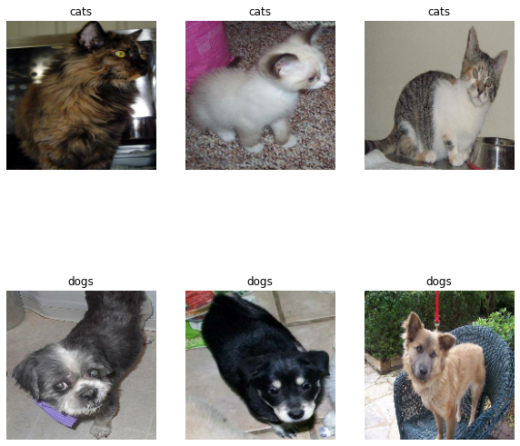
The following code into the next block. This is technical code related to rapidly reading data. Here is related link: here.
AUTOTUNE = tf.data.AUTOTUNE

train_dataset = train_dataset.prefetch(buffer_size=AUTOTUNE)
validation_dataset = validation_dataset.prefetch(buffer_size=AUTOTUNE)
test_dataset = test_dataset.prefetch(buffer_size=AUTOTUNE)
Check Label Frequencies
The following line of code will create an iterator called labels.
abels_iterator = train_dataset.unbatch().map(lambda image, label: label).as_numpy_iterator()
Compute the number of images in the training data with label 0 (corresponding to "cat") and label 1 (corresponding to "dog").
The baseline machine learning model is the model that always guesses the most frequent label. Briefly discuss how accurate the baseline model would be in our case.
We’ll treat this as the benchmark for improvement. Our models should do much better than baseline in order to be considered good data science achievements!
2. First Model
We will usses tf.keras.Sequential to create our first model (give this model the name model1) including at least two MaxPooling2D layers, at least one Flatten layer, at least one Dense layer, and at least one Dropout layer. Then train this model and plot the history of the accuracy on both the training and validation sets.
We should consistently achieve at least 52% validation accuracy in this part
model1 = models.Sequential([
      layers.Conv2D(32, (3, 3), activation='relu', input_shape=(160, 160, 3)), # input image is 160 "pixels" x 160 "pixels"
      layers.MaxPooling2D((2, 2)),
      layers.Conv2D(32, (3, 3), activation='relu'),
      layers.MaxPooling2D((2, 2)),
      layers.Flatten(), # n^2 * 64 length vector

      layers.Dropout(0.2),
      layers.Dense(2) # number of classes in your dataset
])
model1.summary()
Model: "sequential_6"
_________________________________________________________________
 Layer (type)                Output Shape              Param #
=================================================================
 conv2d_6 (Conv2D)           (None, 158, 158, 32)      896

 max_pooling2d_6 (MaxPooling  (None, 79, 79, 32)       0
 2D)

 conv2d_7 (Conv2D)           (None, 77, 77, 32)        9248

 max_pooling2d_7 (MaxPooling  (None, 38, 38, 32)       0
 2D)

 flatten_3 (Flatten)         (None, 46208)             0

 dropout_3 (Dropout)         (None, 46208)             0

 dense_5 (Dense)             (None, 2)                 92418

=================================================================
Total params: 102,562
Trainable params: 102,562
Non-trainable params: 0
_________________________________________________________________
model1.compile(optimizer='adam',
              loss = tf.keras.losses.SparseCategoricalCrossentropy(from_logits=True),
              metrics = ['accuracy'])
history1 = model1.fit(train_dataset,
                     epochs=20, # how many rounds of training to do
                     validation_data = validation_dataset
                     )
Epoch 1/20
63/63 [==============================] - 6s 75ms/step - loss: 20.6239 - accuracy: 0.5050 - val_loss: 0.6973 - val_accuracy: 0.5000
Epoch 2/20
63/63 [==============================] - 5s 73ms/step - loss: 0.6690 - accuracy: 0.5690 - val_loss: 0.7179 - val_accuracy: 0.4963
Epoch 3/20
63/63 [==============================] - 5s 73ms/step - loss: 0.6186 - accuracy: 0.6220 - val_loss: 0.7574 - val_accuracy: 0.5297
Epoch 4/20
63/63 [==============================] - 5s 73ms/step - loss: 0.5636 - accuracy: 0.6695 - val_loss: 0.8170 - val_accuracy: 0.5384
Epoch 5/20
63/63 [==============================] - 5s 73ms/step - loss: 0.4950 - accuracy: 0.7225 - val_loss: 0.8948 - val_accuracy: 0.5421
Epoch 6/20
63/63 [==============================] - 5s 73ms/step - loss: 0.4236 - accuracy: 0.7820 - val_loss: 1.3312 - val_accuracy: 0.5124
Epoch 7/20
63/63 [==============================] - 5s 73ms/step - loss: 0.4016 - accuracy: 0.7940 - val_loss: 1.5880 - val_accuracy: 0.5260
Epoch 8/20
63/63 [==============================] - 5s 75ms/step - loss: 0.3591 - accuracy: 0.8290 - val_loss: 1.1965 - val_accuracy: 0.5421
Epoch 9/20
63/63 [==============================] - 5s 74ms/step - loss: 0.3138 - accuracy: 0.8550 - val_loss: 1.7997 - val_accuracy: 0.5322
Epoch 10/20
63/63 [==============================] - 6s 90ms/step - loss: 0.2847 - accuracy: 0.8735 - val_loss: 1.7190 - val_accuracy: 0.5446
Epoch 11/20
63/63 [==============================] - 5s 82ms/step - loss: 0.2619 - accuracy: 0.8855 - val_loss: 1.7146 - val_accuracy: 0.5569
Epoch 12/20
63/63 [==============================] - 7s 101ms/step - loss: 0.2127 - accuracy: 0.9080 - val_loss: 2.3426 - val_accuracy: 0.5532
Epoch 13/20
63/63 [==============================] - 5s 73ms/step - loss: 0.1907 - accuracy: 0.9205 - val_loss: 2.5349 - val_accuracy: 0.5681
Epoch 14/20
63/63 [==============================] - 5s 73ms/step - loss: 0.2098 - accuracy: 0.9165 - val_loss: 2.3476 - val_accuracy: 0.5408
Epoch 15/20
63/63 [==============================] - 5s 72ms/step - loss: 0.2306 - accuracy: 0.9165 - val_loss: 2.2886 - val_accuracy: 0.5359
Epoch 16/20
63/63 [==============================] - 5s 72ms/step - loss: 0.2570 - accuracy: 0.9105 - val_loss: 2.3505 - val_accuracy: 0.5594
Epoch 17/20
63/63 [==============================] - 5s 72ms/step - loss: 0.2089 - accuracy: 0.9275 - val_loss: 2.5498 - val_accuracy: 0.5532
Epoch 18/20
63/63 [==============================] - 5s 74ms/step - loss: 0.2067 - accuracy: 0.9205 - val_loss: 2.9071 - val_accuracy: 0.5631
Epoch 19/20
63/63 [==============================] - 5s 74ms/step - loss: 0.1853 - accuracy: 0.9360 - val_loss: 2.7934 - val_accuracy: 0.5829
Epoch 20/20
63/63 [==============================] - 5s 75ms/step - loss: 0.1266 - accuracy: 0.9535 - val_loss: 2.9360 - val_accuracy: 0.5644
plt.plot(history1.history["accuracy"], label = "training")
plt.plot(history1.history["val_accuracy"], label = "validation")
plt.gca().set(xlabel = "epoch", ylabel = "accuracy")
plt.legend()
<matplotlib.legend.Legend at 0x7f0e18fc0050>
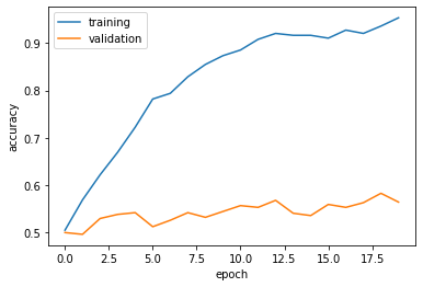
When I build the models, I have one more Dense layer “layers.Dense(64, activation=’relu’)” before the last layer, but it resulting 100% training accuracy but 50% validation accuracy at the end.
I also added layers.Conv2D(64, (3, 3), activation=’relu’), and resulting in a similar result as the above code.
From the outputs, we get some information about the model1:
- The validation accuracy of my model stabilized between 54% and 57% after a few epochs during training, which is 8% better than baseline.
- This model gets approximately 57% validation accuracy, which is 5% higher than the baseline
- Clearly, we have overfitting in model1, as epochs increase, the gap between training accuracy and validation accuracy becomes bigger.
3. Model with Data Augmentation
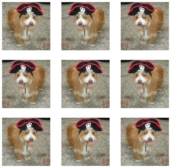
- First, create a tf.keras.layers.RandomFlip() layer. Make a plot of the original image and a few copies to which RandomFlip() has been applied. Make sure to check the documentation for this function!
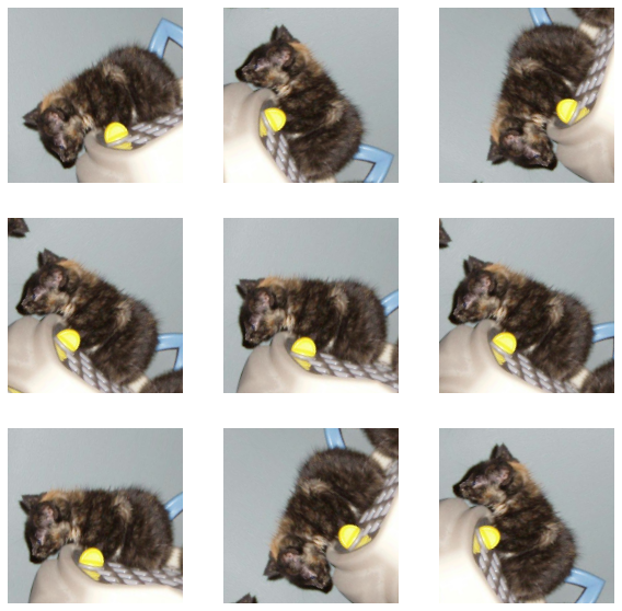
- Next, create a tf.keras.layers.RandomRotation() layer. Check the docs to learn more about the arguments accepted by this layer. Then, make a plot of both the original image and a few copies to which RandomRotation() has been applied.
# random flip
data_augmentation_flip = tf.keras.Sequential([
  tf.keras.layers.RandomFlip('horizontal'),
])

# random rotation
data_augmentation_rotation = tf.keras.Sequential([
  tf.keras.layers.RandomRotation(0.2),
])

# both random flip and random rotation
data_augmentation = tf.keras.Sequential([
  tf.keras.layers.RandomFlip('horizontal'),
  tf.keras.layers.RandomRotation(0.2),
])
Let’s apply filp multiple times on an image:
for image, _ in train_dataset.take(1):
  plt.figure(figsize=(10, 10))
  first_image = image[0]
  for i in range(9):
    ax = plt.subplot(3, 3, i + 1)
    augmented_image = data_augmentation_flip(tf.expand_dims(first_image, 0), training=True)
    plt.imshow(augmented_image[0] / 255)
    plt.axis('off')
Let’s apply rotation multiple times on an image:
for image, _ in train_dataset.take(1):
  plt.figure(figsize=(10, 10))
  first_image = image[0]
  for i in range(9):
    ax = plt.subplot(3, 3, i + 1)
    augmented_image = data_augmentation_rotation(tf.expand_dims(first_image, 0), training=True)
    plt.imshow(augmented_image[0] / 255)
    plt.axis('off')
model2 = models.Sequential([
      data_augmentation, # rotation and flip
      layers.Conv2D(32, (3, 3), activation='relu', input_shape=(160, 160, 3)), # input image is 160 "pixels" x 160 "pixels"
      layers.MaxPooling2D((2, 2)),
      layers.Conv2D(32, (3, 3), activation='relu'),
      layers.MaxPooling2D((2, 2)),
      layers.Dropout(0.2),
      layers.Flatten(), # n^2 * 64 length vector

      layers.Dense(64, activation='relu'),
      layers.Dense(2) # number of classes in your dataset
])
model2.compile(optimizer='adam',
              loss = tf.keras.losses.SparseCategoricalCrossentropy(from_logits=True),
              metrics = ['accuracy'])
history2 = model2.fit(train_dataset,
                     epochs=20, # how many rounds of training to do
                     validation_data = validation_dataset
                     )
Epoch 1/20
63/63 [==============================] - 7s 78ms/step - loss: 69.1872 - accuracy: 0.5180 - val_loss: 0.7004 - val_accuracy: 0.5470
Epoch 2/20
63/63 [==============================] - 5s 77ms/step - loss: 0.6965 - accuracy: 0.5570 - val_loss: 0.7016 - val_accuracy: 0.5569
Epoch 3/20
63/63 [==============================] - 6s 91ms/step - loss: 0.6885 - accuracy: 0.5550 - val_loss: 0.6881 - val_accuracy: 0.5260
Epoch 4/20
63/63 [==============================] - 6s 86ms/step - loss: 0.6864 - accuracy: 0.5535 - val_loss: 0.6986 - val_accuracy: 0.5248
Epoch 5/20
63/63 [==============================] - 6s 97ms/step - loss: 0.6822 - accuracy: 0.5665 - val_loss: 0.7039 - val_accuracy: 0.5569
Epoch 6/20
63/63 [==============================] - 5s 77ms/step - loss: 0.6810 - accuracy: 0.5675 - val_loss: 0.7059 - val_accuracy: 0.5347
Epoch 7/20
63/63 [==============================] - 5s 76ms/step - loss: 0.6846 - accuracy: 0.5380 - val_loss: 0.7031 - val_accuracy: 0.5322
Epoch 8/20
63/63 [==============================] - 5s 76ms/step - loss: 0.6779 - accuracy: 0.5775 - val_loss: 0.7130 - val_accuracy: 0.5520
Epoch 9/20
63/63 [==============================] - 5s 76ms/step - loss: 0.6807 - accuracy: 0.5595 - val_loss: 0.7185 - val_accuracy: 0.5111
Epoch 10/20
63/63 [==============================] - 5s 76ms/step - loss: 0.6703 - accuracy: 0.6050 - val_loss: 0.7173 - val_accuracy: 0.5557
Epoch 11/20
63/63 [==============================] - 5s 76ms/step - loss: 0.6826 - accuracy: 0.5635 - val_loss: 0.7128 - val_accuracy: 0.5050
Epoch 12/20
63/63 [==============================] - 5s 76ms/step - loss: 0.6680 - accuracy: 0.5940 - val_loss: 0.6998 - val_accuracy: 0.5582
Epoch 13/20
63/63 [==============================] - 5s 76ms/step - loss: 0.6818 - accuracy: 0.5610 - val_loss: 0.6861 - val_accuracy: 0.5718
Epoch 14/20
63/63 [==============================] - 5s 75ms/step - loss: 0.6780 - accuracy: 0.5580 - val_loss: 0.7109 - val_accuracy: 0.5483
Epoch 15/20
63/63 [==============================] - 5s 75ms/step - loss: 0.6791 - accuracy: 0.5790 - val_loss: 0.7068 - val_accuracy: 0.4963
Epoch 16/20
63/63 [==============================] - 5s 76ms/step - loss: 0.6829 - accuracy: 0.5545 - val_loss: 0.6950 - val_accuracy: 0.5582
Epoch 17/20
63/63 [==============================] - 5s 76ms/step - loss: 0.6782 - accuracy: 0.5720 - val_loss: 0.7095 - val_accuracy: 0.5495
Epoch 18/20
63/63 [==============================] - 5s 76ms/step - loss: 0.6723 - accuracy: 0.5885 - val_loss: 0.7156 - val_accuracy: 0.5396
Epoch 19/20
63/63 [==============================] - 5s 76ms/step - loss: 0.6579 - accuracy: 0.5895 - val_loss: 0.7274 - val_accuracy: 0.5532
Epoch 20/20
63/63 [==============================] - 5s 75ms/step - loss: 0.6601 - accuracy: 0.6050 - val_loss: 0.7292 - val_accuracy: 0.5507
plt.plot(history2.history["accuracy"], label = "training")
plt.plot(history2.history["val_accuracy"], label = "validation")
plt.gca().set(xlabel = "epoch", ylabel = "accuracy")
plt.legend()
<matplotlib.legend.Legend at 0x7f0d9f9ea290>
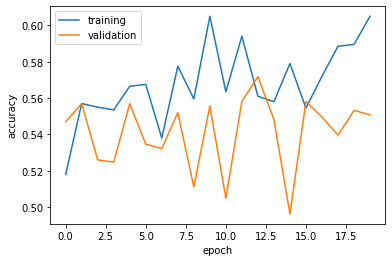
In this models, I add/remove Dense layer “layers.Dense(64, activation=’relu’)”, add one more “drop layer”, and also adjust the degree of rotation or direction of flip in argumation. In most case, we are getting worse result:
- The validation accuracy of my model stabilized between 55% and 57%, which is 4% higher the baseline on average.
- On average, this model gets approximately 50% validation accuracy, which is lower than the model1
- Our model in this section performs a bit worse than the one before, even on the validation set. I ran this model for about 20 times with adding or remove different layers, the best case that I got is 59% validation accuracy. But, we can see the overfitting in model2 are reduced a lot compare to model1, the gap between training accuracy and validation accuracy is 2%. So model2 dont have or have very small overfitting problem.
4. Data Preprocessing
Sometimes, it can be helpful to make simple transformations to the input data. For example, in this case, the original data has pixels with RGB values between 0 and 255, but many models will train faster with RGB values normalized between 0 and 1, or possibly between -1 and 1. These are mathematically identical situations, since we can always just scale the weights. But if we handle the scaling prior to the training process, we can spend more of our training energy handling actual signal in the data and less energy having the weights adjust to the data scale.
The following code will create a preprocessing layer called preprocessor which you can slot into your model pipeline.
i = tf.keras.Input(shape=(160, 160, 3))
x = tf.keras.applications.mobilenet_v2.preprocess_input(i)
preprocessor = tf.keras.Model(inputs = [i], outputs = [x])
I suggest incorporating the preprocessor layer as the very first layer, before the data augmentation layers.
model3 = models.Sequential([
      preprocessor, #  simple transformations to the input data
      data_augmentation, # rotation and flip
      layers.Conv2D(32, (3, 3), activation='relu', input_shape=(160, 160, 3)), # input image is 160 "pixels" x 160 "pixels"
      layers.MaxPooling2D((2, 2)),
      layers.Conv2D(32, (3, 3), activation='relu'),
      layers.MaxPooling2D((2, 2)),
      layers.Dropout(0.2),
      layers.Flatten(), # n^2 * 64 length vector

      layers.Dense(64, activation='relu'),
      layers.Dense(2) # number of classes in your dataset
])
model3.compile(optimizer='adam',
              loss = tf.keras.losses.SparseCategoricalCrossentropy(from_logits=True),
              metrics = ['accuracy'])
model3.summary()
Model: "sequential_15"
_________________________________________________________________
 Layer (type)                Output Shape              Param #
=================================================================
 model_1 (Functional)        (None, 160, 160, 3)       0

 sequential_9 (Sequential)   (None, 160, 160, 3)       0

 conv2d_18 (Conv2D)          (None, 158, 158, 32)      896

 max_pooling2d_18 (MaxPoolin  (None, 79, 79, 32)       0
 g2D)

 conv2d_19 (Conv2D)          (None, 77, 77, 32)        9248

 max_pooling2d_19 (MaxPoolin  (None, 38, 38, 32)       0
 g2D)

 dropout_9 (Dropout)         (None, 38, 38, 32)        0

 flatten_9 (Flatten)         (None, 46208)             0

 dense_16 (Dense)            (None, 64)                2957376

 dense_17 (Dense)            (None, 2)                 130

=================================================================
Total params: 2,967,650
Trainable params: 2,967,650
Non-trainable params: 0
_________________________________________________________________
history3 = model3.fit(train_dataset,
                     epochs=20, # how many rounds of training to do
                     validation_data = validation_dataset
                     )
Epoch 1/20
63/63 [==============================] - 6s 78ms/step - loss: 0.8475 - accuracy: 0.5225 - val_loss: 0.6666 - val_accuracy: 0.5495
Epoch 2/20
63/63 [==============================] - 5s 76ms/step - loss: 0.6654 - accuracy: 0.5920 - val_loss: 0.6211 - val_accuracy: 0.6225
Epoch 3/20
63/63 [==============================] - 5s 77ms/step - loss: 0.6350 - accuracy: 0.6270 - val_loss: 0.6417 - val_accuracy: 0.6176
Epoch 4/20
63/63 [==============================] - 5s 77ms/step - loss: 0.6321 - accuracy: 0.6465 - val_loss: 0.6205 - val_accuracy: 0.6436
Epoch 5/20
63/63 [==============================] - 5s 75ms/step - loss: 0.6057 - accuracy: 0.6485 - val_loss: 0.6103 - val_accuracy: 0.6708
Epoch 6/20
63/63 [==============================] - 5s 76ms/step - loss: 0.5876 - accuracy: 0.6800 - val_loss: 0.5874 - val_accuracy: 0.6609
Epoch 7/20
63/63 [==============================] - 5s 76ms/step - loss: 0.5858 - accuracy: 0.6970 - val_loss: 0.5939 - val_accuracy: 0.6943
Epoch 8/20
63/63 [==============================] - 5s 76ms/step - loss: 0.5780 - accuracy: 0.6785 - val_loss: 0.5782 - val_accuracy: 0.6881
Epoch 9/20
63/63 [==============================] - 5s 76ms/step - loss: 0.5732 - accuracy: 0.6960 - val_loss: 0.5592 - val_accuracy: 0.7141
Epoch 10/20
63/63 [==============================] - 5s 77ms/step - loss: 0.5533 - accuracy: 0.7155 - val_loss: 0.5594 - val_accuracy: 0.7054
Epoch 11/20
63/63 [==============================] - 5s 79ms/step - loss: 0.5461 - accuracy: 0.7110 - val_loss: 0.5745 - val_accuracy: 0.6869
Epoch 12/20
63/63 [==============================] - 5s 78ms/step - loss: 0.5538 - accuracy: 0.7065 - val_loss: 0.5589 - val_accuracy: 0.7191
Epoch 13/20
63/63 [==============================] - 5s 79ms/step - loss: 0.5199 - accuracy: 0.7365 - val_loss: 0.5624 - val_accuracy: 0.7017
Epoch 14/20
63/63 [==============================] - 5s 78ms/step - loss: 0.5153 - accuracy: 0.7360 - val_loss: 0.5839 - val_accuracy: 0.7079
Epoch 15/20
63/63 [==============================] - 5s 79ms/step - loss: 0.5243 - accuracy: 0.7310 - val_loss: 0.5547 - val_accuracy: 0.7178
Epoch 16/20
63/63 [==============================] - 5s 79ms/step - loss: 0.4880 - accuracy: 0.7555 - val_loss: 0.5509 - val_accuracy: 0.7228
Epoch 17/20
63/63 [==============================] - 5s 79ms/step - loss: 0.4935 - accuracy: 0.7700 - val_loss: 0.5287 - val_accuracy: 0.7351
Epoch 18/20
63/63 [==============================] - 5s 79ms/step - loss: 0.4865 - accuracy: 0.7595 - val_loss: 0.5276 - val_accuracy: 0.7327
Epoch 19/20
63/63 [==============================] - 5s 77ms/step - loss: 0.4819 - accuracy: 0.7715 - val_loss: 0.5190 - val_accuracy: 0.7525
Epoch 20/20
63/63 [==============================] - 5s 79ms/step - loss: 0.4766 - accuracy: 0.7570 - val_loss: 0.5467 - val_accuracy: 0.7228
plt.plot(history3.history["accuracy"], label = "training")
plt.plot(history3.history["val_accuracy"], label = "validation")
plt.gca().set(xlabel = "epoch", ylabel = "accuracy")
plt.legend()
<matplotlib.legend.Legend at 0x7f0da029ad90>
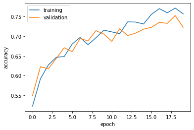
- The validation accuracy of my model stabilized between 70% and 72%, which is 10% higher the baseline on average.
- On average, this model gets approximately 70% validation accuracy, which is 15% higher than the model1
- On the graph, we can see the accuracy for training and validation are really closed which indicate we dont have overfitting issue for model3.
5. Transfer Learning
So far, we’ve been training models for distinguishing between cats and dogs from scratch. In some cases, however, someone might already have trained a model that does a related task, and might have learned some relevant patterns. For example, folks train machine learning models for a variety of image recognition tasks. Maybe we could use a pre-existing model for our task?
To do this, we need to first access a pre-existing “base model”, incorporate it into a full model for our current task, and then train that model.
Paste the following code in order to download MobileNetV2 and configure it as a layer that can be included in your model.
IMG_SHAPE = IMG_SIZE + (3,)
base_model = tf.keras.applications.MobileNetV2(input_shape=IMG_SHAPE,
                                               include_top=False,
                                               weights='imagenet')
base_model.trainable = False

i = tf.keras.Input(shape=IMG_SHAPE)
x = base_model(i, training = False)
base_model_layer = tf.keras.Model(inputs = [i], outputs = [x])
Downloading data from https://storage.googleapis.com/tensorflow/keras-applications/mobilenet_v2/mobilenet_v2_weights_tf_dim_ordering_tf_kernels_1.0_160_no_top.h5
9412608/9406464 [==============================] - 0s 0us/step
9420800/9406464 [==============================] - 0s 0us/step
model4 = models.Sequential([
      preprocessor, #  simple transformations to the input data
      data_augmentation, # rotation and flip
      base_model_layer,
      layers.GlobalMaxPool2D(),
      layers.Dropout(0.2),
      layers.Flatten(), # n^2 * 64 length vector

      layers.Dense(64, activation='relu'),
      layers.Dense(2) # number of classes in your dataset
])
model4.compile(optimizer='adam',
              loss = tf.keras.losses.SparseCategoricalCrossentropy(from_logits=True),
              metrics = ['accuracy'])
model4.summary()
Model: "sequential_16"
_________________________________________________________________
 Layer (type)                Output Shape              Param #
=================================================================
 model_1 (Functional)        (None, 160, 160, 3)       0

 sequential_9 (Sequential)   (None, 160, 160, 3)       0

 model_2 (Functional)        (None, 5, 5, 1280)        2257984

 global_max_pooling2d (Globa  (None, 1280)             0
 lMaxPooling2D)

 dropout_10 (Dropout)        (None, 1280)              0

 flatten_10 (Flatten)        (None, 1280)              0

 dense_18 (Dense)            (None, 64)                81984

 dense_19 (Dense)            (None, 2)                 130

=================================================================
Total params: 2,340,098
Trainable params: 82,114
Non-trainable params: 2,257,984
_________________________________________________________________
For the base_model_layer, we have 2257984 parameters to train, which is quite a big number.
history4 = model4.fit(train_dataset,
                     epochs=20, # how many rounds of training to do
                     validation_data = validation_dataset
                     )
Epoch 1/20
63/63 [==============================] - 11s 114ms/step - loss: 0.7686 - accuracy: 0.8430 - val_loss: 0.0695 - val_accuracy: 0.9715
Epoch 2/20
63/63 [==============================] - 6s 85ms/step - loss: 0.2151 - accuracy: 0.9175 - val_loss: 0.0623 - val_accuracy: 0.9740
Epoch 3/20
63/63 [==============================] - 6s 86ms/step - loss: 0.1947 - accuracy: 0.9215 - val_loss: 0.0565 - val_accuracy: 0.9839
Epoch 4/20
63/63 [==============================] - 6s 84ms/step - loss: 0.1579 - accuracy: 0.9325 - val_loss: 0.0751 - val_accuracy: 0.9641
Epoch 5/20
63/63 [==============================] - 6s 85ms/step - loss: 0.1538 - accuracy: 0.9350 - val_loss: 0.0546 - val_accuracy: 0.9839
Epoch 6/20
63/63 [==============================] - 6s 87ms/step - loss: 0.1565 - accuracy: 0.9370 - val_loss: 0.0534 - val_accuracy: 0.9740
Epoch 7/20
63/63 [==============================] - 6s 86ms/step - loss: 0.1372 - accuracy: 0.9465 - val_loss: 0.0585 - val_accuracy: 0.9777
Epoch 8/20
63/63 [==============================] - 6s 86ms/step - loss: 0.1279 - accuracy: 0.9495 - val_loss: 0.0557 - val_accuracy: 0.9765
Epoch 9/20
63/63 [==============================] - 6s 85ms/step - loss: 0.1244 - accuracy: 0.9475 - val_loss: 0.0442 - val_accuracy: 0.9851
Epoch 10/20
63/63 [==============================] - 6s 97ms/step - loss: 0.1040 - accuracy: 0.9555 - val_loss: 0.0452 - val_accuracy: 0.9876
Epoch 11/20
63/63 [==============================] - 6s 86ms/step - loss: 0.1253 - accuracy: 0.9440 - val_loss: 0.0474 - val_accuracy: 0.9802
Epoch 12/20
63/63 [==============================] - 6s 86ms/step - loss: 0.1047 - accuracy: 0.9575 - val_loss: 0.0530 - val_accuracy: 0.9814
Epoch 13/20
63/63 [==============================] - 6s 85ms/step - loss: 0.1158 - accuracy: 0.9575 - val_loss: 0.0505 - val_accuracy: 0.9802
Epoch 14/20
63/63 [==============================] - 6s 87ms/step - loss: 0.1183 - accuracy: 0.9495 - val_loss: 0.0481 - val_accuracy: 0.9814
Epoch 15/20
63/63 [==============================] - 6s 87ms/step - loss: 0.1032 - accuracy: 0.9600 - val_loss: 0.0470 - val_accuracy: 0.9814
Epoch 16/20
63/63 [==============================] - 6s 85ms/step - loss: 0.1052 - accuracy: 0.9555 - val_loss: 0.0434 - val_accuracy: 0.9827
Epoch 17/20
63/63 [==============================] - 6s 85ms/step - loss: 0.1088 - accuracy: 0.9570 - val_loss: 0.0426 - val_accuracy: 0.9876
Epoch 18/20
63/63 [==============================] - 6s 86ms/step - loss: 0.0934 - accuracy: 0.9620 - val_loss: 0.0386 - val_accuracy: 0.9802
Epoch 19/20
63/63 [==============================] - 6s 86ms/step - loss: 0.0798 - accuracy: 0.9720 - val_loss: 0.0427 - val_accuracy: 0.9827
Epoch 20/20
63/63 [==============================] - 6s 86ms/step - loss: 0.0822 - accuracy: 0.9665 - val_loss: 0.0443 - val_accuracy: 0.9864
plt.plot(history4.history["accuracy"], label = "training")
plt.plot(history4.history["val_accuracy"], label = "validation")
plt.gca().set(xlabel = "epoch", ylabel = "accuracy")
plt.legend()
<matplotlib.legend.Legend at 0x7f0d9fa97a10>
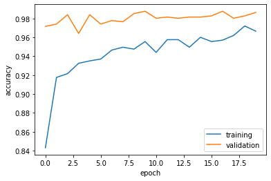
- The validation accuracy of my model stabilized between 97% and 98%, which is 47% higher the baseline on average.
- On average, this model gets approximately 97.5% validation accuracy, which is 42% higher than the model1
- On the graph, we can see the accuracy for training and validation are close to each other when epochs increases, the overfitting problem is reducing when epochs increasing.
6. Score on Test Data
model4.evaluate(test_dataset)
6/6 [==============================] - 1s 67ms/step - loss: 0.0167 - accuracy: 0.9948
[0.016668593510985374, 0.9947916865348816]
The average accuracy for testing data is 99%, that’s a pretty good number for the testing result.