Fake News Classification by NLP
Blog Post: Fake News Classification
Rampant misinformation—often called “fake news”—is one of the defining features of contemporary democratic life. In this Blog Post, we will develop and assess a fake news classifier using Tensorflow.
Data Source
Our data for this assignment comes from the article
Ahmed H, Traore I, Saad S. (2017) “Detection of Online Fake News Using N-Gram Analysis and Machine Learning Techniques. In: Traore I., Woungang I., Awad A. (eds) Intelligent, Secure, and Dependable Systems in Distributed and Cloud Environments. ISDDC 2017. Lecture Notes in Computer Science, vol 10618. Springer, Cham (pp. 127-138).
1 Acquire Training Data
The data been hosted at the below URL:
import numpy as np
import pandas as pd
import tensorflow as tf
import re
import string

from tensorflow.keras import layers
from tensorflow.keras import losses
from tensorflow import keras

# requires update to tensorflow 2.4
# >>> conda activate PIC16B
# >>> pip install tensorflow==2.4
from tensorflow.keras.layers.experimental.preprocessing import TextVectorization
from tensorflow.keras.layers.experimental.preprocessing import StringLookup

from sklearn.model_selection import train_test_split
from sklearn.preprocessing import LabelEncoder

# for embedding viz
import plotly.express as px
import plotly.io as pio
pio.templates.default = "plotly_white"
train_url = "https://github.com/PhilChodrow/PIC16b/blob/master/datasets/fake_news_train.csv?raw=true"
df_train = pd.read_csv(train_url)
df_train.head()
| Unnamed: 0 | title | text | fake | |
|---|---|---|---|---|
| 0 | 17366 | Merkel: Strong result for Austria's FPO 'big c... | German Chancellor Angela Merkel said on Monday... | 0 |
| 1 | 5634 | Trump says Pence will lead voter fraud panel | WEST PALM BEACH, Fla.President Donald Trump sa... | 0 |
| 2 | 17487 | JUST IN: SUSPECTED LEAKER and “Close Confidant... | On December 5, 2017, Circa s Sara Carter warne... | 1 |
| 3 | 12217 | Thyssenkrupp has offered help to Argentina ove... | Germany s Thyssenkrupp, has offered assistance... | 0 |
| 4 | 5535 | Trump say appeals court decision on travel ban... | President Donald Trump on Thursday called the ... | 0 |
le = LabelEncoder()
df_train["fake"] = le.fit_transform(df_train["fake"])
num_fake = len(df_train["fake"].unique())
- Each row of the data corresponds to an article.
- The title column gives the title of the article, while the text column gives the full article text.
- The final column, called fake, is 0 if the article is true and 1 if the article contains fake news, as determined by the authors of the paper above.
2. Make a Dataset
Write a function called make_dataset. This function should do two things:
- Remove stopwords from the article text and title. A stopword is a word that is usually considered to be uninformative, such as “the,” “and,” or “but.” Helpful link: StackOverFlow thread
- Construct and return a tf.data.Dataset with two inputs and one output. The input should be of the form (title, text), and the output should consist only of the fake column. This tutorial for reference on how to construct and use Datasets with multiple inputs.
import nltk
from nltk.corpus import stopwords
nltk.download('stopwords')
stop = stopwords.words('english')

'''
function takes a data frame as input, then remove stop words of the dataframe with column names title and text.
next the function use processed dataframe to make a rf.data.dataset object and return it.
'''
def make_dataset(df):
  # remove stopwords for column
  # Exclude stopwords with Python's list comprehension and pandas.DataFrame.apply.
  df['title'] = df['title'].apply(lambda x: ' '.join([word for word in x.split() if word not in (stop)]))
  df['text'] = df['text'].apply(lambda x: ' '.join([word for word in x.split() if word not in (stop)]))

  data = tf.data.Dataset.from_tensor_slices((
      # dictionary for input data/features
      {'title': df[['title']],
       'text': df[['text']]},
       # dictionary for output data/labels
      {'fake': df['fake']}
      ))

  return data
[nltk_data] Downloading package stopwords to /root/nltk_data...
[nltk_data]   Package stopwords is already up-to-date!
df_new = make_dataset(df_train)
validation data
split of 20% of the new dataset we made to use for validation.
df_new = df_new.shuffle(buffer_size = len(df_new))

train_size = int(0.8*len(df_new)) # 80% training size
val_size   = int(0.2*len(df_new)) # 20% validation size

train = df_new.take(train_size).batch(20) # grouping into 20s, makes trainning faster
val = df_new.skip(train_size).take(val_size).batch(20)

print(len(train), len(val))
898 225
Base Rate
Recall that the base rate refers to the accuracy of a model that always makes the same guess (for example, such a model might always say “fake news!”). The base rate for this data set by examining the labels on the training set.
When we determine wether a news is fake news or not, without any new or interesting occurs to impact the outcome. The rate of a news is a fake news is 52% on the trainning data set which the base rate for this model is 52%.
sum(df_train["fake"] == 1)/len(df_train)
0.522963160942581
TextVectorization
Here is one option:
#preparing a text vectorization layer for tf model
size_vocabulary = 2000

def standardization(input_data):
    lowercase = tf.strings.lower(input_data)
    no_punctuation = tf.strings.regex_replace(lowercase,
                                  '[%s]' % re.escape(string.punctuation),'')
    return no_punctuation

title_vectorize_layer = TextVectorization(
    standardize=standardization,
    max_tokens=size_vocabulary, # only consider this many words
    output_mode='int', # get frequency ranking for each word in the training dataset
    output_sequence_length=500)

title_vectorize_layer.adapt(train.map(lambda x, y: x["title"]))
title_input = keras.Input(
    shape=(1,),
    name = "title", # same name as the dictionary key in the dataset
    dtype = "string"
)

text_input = keras.Input(
    shape=(1, ),
    name = "text",
    dtype = "string"
)
3. Create Models
Use TensorFlow models to offer a perspective on the following question:
When detecting fake news, is it most effective to focus on only the title of the article, the full text of the article, or both?
To address this question, create three (3) TensorFlow models.
- In the first model, use only the article title as an input.
- In the second model, use only the article text as an input.
- In the third model, use both the article title and the article text as input.
Train our models on the training data until they appear to be “fully” trained. Assess and compare their performance. Make sure to include a visualization of the training histories.
We can visualize our models with this code:
from tensorflow.keras import utils
utils.plot_model(model)
Notes
- For the first two models, we don’t have to create new Datasets. Instead, just specify the inputs to the keras.Model appropriately, and TensorFlow will automatically ignore the unused inputs in the Dataset.
- The lecture notes and tutorials linked above are likely to be helpful as we are creating our models as well.
- We will need to use the Functional API, rather than the Sequential API, for this modeling task.
- When using the Functional API, it is possible to use the same layer in multiple parts of our model; see this tutorial for examples. I recommended that we share an embedding layer for both the article title and text inputs. We may encounter overfitting, in which case Dropout layers can help.
We’re free to be creative when designing our models. If we’re feeling very stuck, start with some of the pipelines for processing text that we’ve seen in lecture, and iterate from there. Please include in our discussion some of the things that we tried and how we determined the models we used.
What Accuracy Should We Aim For?
Our three different models might have noticeably different performance. Our best model should be able to consistently score at least 97% validation accuracy.
After comparing the performance of each model on validation data, make a recommendation regarding the question at the beginning of this section. Should algorithms use the title, the text, or both when seeking to detect fake news?
# title layer
title_features = title_vectorize_layer(title_input) # apply this "function TextVectorization layer" to lyrics_input
title_features = layers.Embedding(size_vocabulary, output_dim = 2, name="embedding1")(title_features)
title_features = layers.Dropout(0.2)(title_features)
title_features = layers.GlobalAveragePooling1D()(title_features)
title_features = layers.Dropout(0.2)(title_features)
title_features = layers.Dense(32, activation='relu')(title_features)

# for model1 (title input only)
title_features= layers.Dense(32, activation='relu')(title_features)
output1 = layers.Dense(num_fake , name="fake")(title_features)

# text layer
text_features = title_vectorize_layer(text_input) # apply this "function TextVectorization layer" to lyrics_input
text_features = layers.Embedding(size_vocabulary, output_dim = 2, name="embedding2")(text_features)
text_features = layers.Dropout(0.2)(text_features)
text_features = layers.GlobalAveragePooling1D()(text_features)
text_features = layers.Dropout(0.2)(text_features)
text_features = layers.Dense(32, activation='relu')(text_features)

# for model2 (text input only)
text_features= layers.Dense(32, activation='relu')(text_features)
output2 = layers.Dense(num_fake , name="fake")(text_features)

# for model3 (both title and text)
main = layers.concatenate([title_features, text_features], axis = 1)
main = layers.Dense(32, activation='relu')(main)
output3 = layers.Dense(num_fake, name="fake")(main)
model1 = keras.Model(
    inputs = title_input,
    outputs = output1
)

model2 = keras.Model(
    inputs = text_input,
    outputs = output2
)

model3 = keras.Model(
    inputs = [title_input, text_input],
    outputs = output3
)
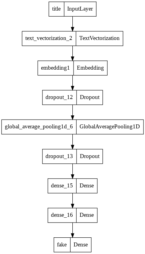
model 1
model1.summary()
Model: "model_9"
_________________________________________________________________
 Layer (type)                Output Shape              Param #
=================================================================
 title (InputLayer)          [(None, 1)]               0

 text_vectorization_2 (TextV  (None, 500)              0
 ectorization)

 embedding1 (Embedding)      (None, 500, 2)            4000

 dropout_12 (Dropout)        (None, 500, 2)            0

 global_average_pooling1d_6   (None, 2)                0
 (GlobalAveragePooling1D)

 dropout_13 (Dropout)        (None, 2)                 0

 dense_15 (Dense)            (None, 32)                96

 dense_16 (Dense)            (None, 32)                1056

 fake (Dense)                (None, 2)                 66

=================================================================
Total params: 5,218
Trainable params: 5,218
Non-trainable params: 0
_________________________________________________________________
keras.utils.plot_model(model1)
model1.compile(optimizer="adam",
              loss = losses.SparseCategoricalCrossentropy(from_logits=True),
              metrics=["accuracy"])
history1 = model1.fit(train,
                    validation_data=val,
                    epochs = 50,
                    verbose = False)
/usr/local/lib/python3.7/dist-packages/keras/engine/functional.py:559: UserWarning:

Input dict contained keys ['text'] which did not match any model input. They will be ignored by the model.
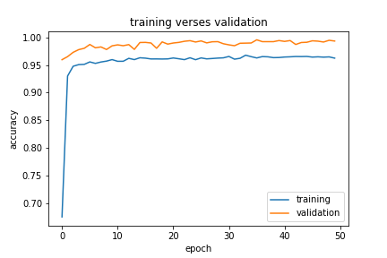
table1 = pd.DataFrame({'accuracy' : history1.history["accuracy"], 'val_accuracy' : history1.history["val_accuracy"]})
table1[29:] # last 20 epochs
| accuracy | val_accuracy | |
|---|---|---|
| 29 | 0.965031 | 0.995099 |
| 30 | 0.960354 | 0.993317 |
| 31 | 0.961523 | 0.989753 |
| 32 | 0.964308 | 0.988416 |
| 33 | 0.962860 | 0.984184 |
| 34 | 0.961078 | 0.991980 |
| 35 | 0.964196 | 0.994208 |
| 36 | 0.964753 | 0.992426 |
| 37 | 0.964308 | 0.993317 |
| 38 | 0.963862 | 0.992649 |
| 39 | 0.967537 | 0.986411 |
| 40 | 0.963974 | 0.993985 |
| 41 | 0.964141 | 0.987302 |
| 42 | 0.963584 | 0.994876 |
| 43 | 0.965811 | 0.993763 |
| 44 | 0.965087 | 0.984629 |
| 45 | 0.963639 | 0.988416 |
| 46 | 0.965310 | 0.988862 |
| 47 | 0.963194 | 0.990198 |
| 48 | 0.965978 | 0.993540 |
| 49 | 0.965644 | 0.995099 |
from matplotlib import pyplot as plt
plt.plot(history1.history["accuracy"], label = "training")
plt.plot(history1.history["val_accuracy"], label = "validation")
plt.gca().set(xlabel = "epoch", ylabel = "accuracy")
plt.title("training verses validation")
plt.legend()
[<matplotlib.lines.Line2D at 0x7fb300037b10>]
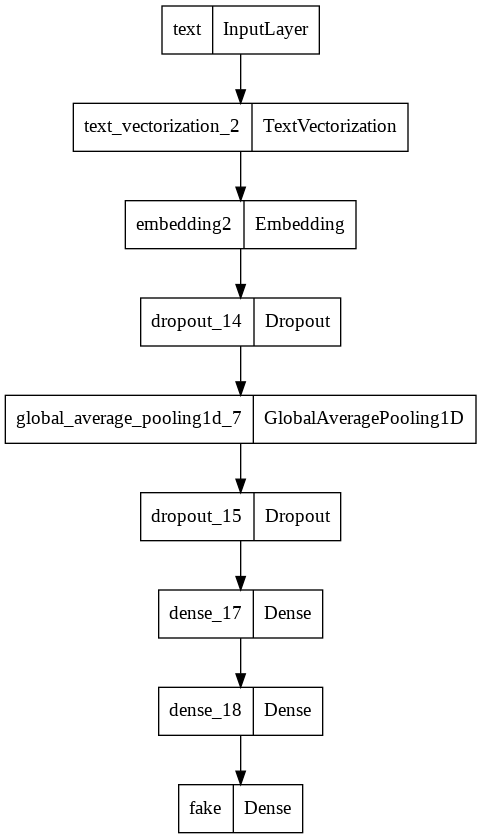
model 2
model2.summary()
Model: "model_10"
_________________________________________________________________
 Layer (type)                Output Shape              Param #
=================================================================
 text (InputLayer)           [(None, 1)]               0

 text_vectorization_2 (TextV  (None, 500)              0
 ectorization)

 embedding2 (Embedding)      (None, 500, 2)            4000

 dropout_14 (Dropout)        (None, 500, 2)            0

 global_average_pooling1d_7   (None, 2)                0
 (GlobalAveragePooling1D)

 dropout_15 (Dropout)        (None, 2)                 0

 dense_17 (Dense)            (None, 32)                96

 dense_18 (Dense)            (None, 32)                1056

 fake (Dense)                (None, 2)                 66

=================================================================
Total params: 5,218
Trainable params: 5,218
Non-trainable params: 0
_________________________________________________________________
keras.utils.plot_model(model2)
model2.compile(optimizer="adam",
              loss = losses.SparseCategoricalCrossentropy(from_logits=True),
              metrics=["accuracy"])
history2 = model2.fit(train,
                    validation_data=val,
                    epochs = 50,
                    verbose = False)
/usr/local/lib/python3.7/dist-packages/keras/engine/functional.py:559: UserWarning:

Input dict contained keys ['title'] which did not match any model input. They will be ignored by the model.
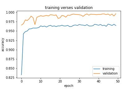
table2 = pd.DataFrame({'accuracy' : history2.history["accuracy"], 'val_accuracy' : history2.history["val_accuracy"]})
table2[29:]  # last 20 epochs
| accuracy | val_accuracy | |
|---|---|---|
| 29 | 0.965755 | 0.991980 |
| 30 | 0.965477 | 0.991980 |
| 31 | 0.965644 | 0.994654 |
| 32 | 0.964809 | 0.994208 |
| 33 | 0.966312 | 0.996213 |
| 34 | 0.964029 | 0.995322 |
| 35 | 0.966813 | 0.994876 |
| 36 | 0.965254 | 0.993763 |
| 37 | 0.966368 | 0.993540 |
| 38 | 0.966312 | 0.994876 |
| 39 | 0.963806 | 0.992649 |
| 40 | 0.968094 | 0.972822 |
| 41 | 0.965811 | 0.993094 |
| 42 | 0.964976 | 0.996213 |
| 43 | 0.966869 | 0.991758 |
| 44 | 0.965811 | 0.993094 |
| 45 | 0.965922 | 0.995767 |
| 46 | 0.965310 | 0.992649 |
| 47 | 0.966702 | 0.995990 |
| 48 | 0.968150 | 0.995322 |
| 49 | 0.964642 | 0.996659 |
plt.plot(history2.history["accuracy"], label = "training")
plt.plot(history2.history["val_accuracy"], label = "validation")
plt.gca().set(xlabel = "epoch", ylabel = "accuracy")
plt.title("training verses validation")
plt.legend()
[<matplotlib.lines.Line2D at 0x7fb2fcfe3210>]
model 3
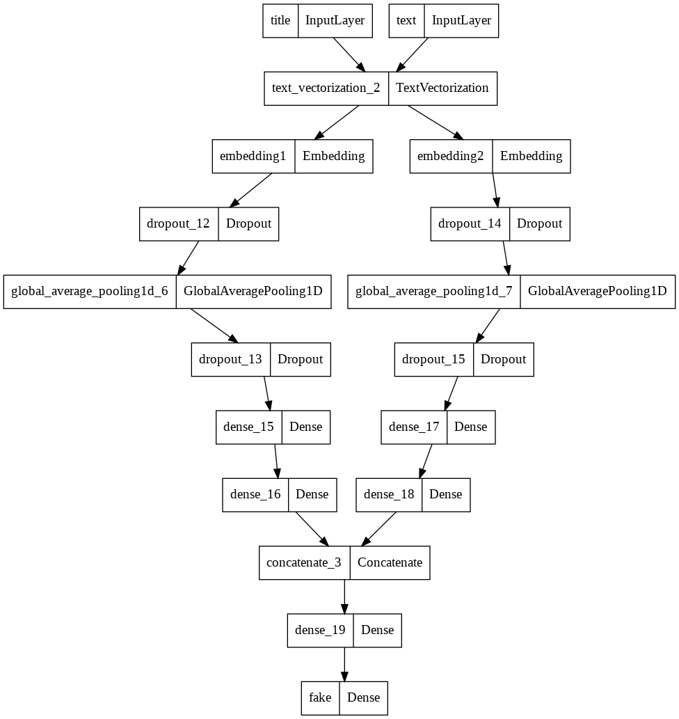
model3.summary()
Model: "model_11"
__________________________________________________________________________________________________
 Layer (type)                   Output Shape         Param #     Connected to
==================================================================================================
 title (InputLayer)             [(None, 1)]          0           []

 text (InputLayer)              [(None, 1)]          0           []

 text_vectorization_2 (TextVect  (None, 500)         0           ['title[0][0]',
 orization)                                                       'text[0][0]']

 embedding1 (Embedding)         (None, 500, 2)       4000        ['text_vectorization_2[0][0]']

 embedding2 (Embedding)         (None, 500, 2)       4000        ['text_vectorization_2[1][0]']

 dropout_12 (Dropout)           (None, 500, 2)       0           ['embedding1[0][0]']

 dropout_14 (Dropout)           (None, 500, 2)       0           ['embedding2[0][0]']

 global_average_pooling1d_6 (Gl  (None, 2)           0           ['dropout_12[0][0]']
 obalAveragePooling1D)

 global_average_pooling1d_7 (Gl  (None, 2)           0           ['dropout_14[0][0]']
 obalAveragePooling1D)

 dropout_13 (Dropout)           (None, 2)            0           ['global_average_pooling1d_6[0][0
                                                                 ]']

 dropout_15 (Dropout)           (None, 2)            0           ['global_average_pooling1d_7[0][0
                                                                 ]']

 dense_15 (Dense)               (None, 32)           96          ['dropout_13[0][0]']

 dense_17 (Dense)               (None, 32)           96          ['dropout_15[0][0]']

 dense_16 (Dense)               (None, 32)           1056        ['dense_15[0][0]']

 dense_18 (Dense)               (None, 32)           1056        ['dense_17[0][0]']

 concatenate_3 (Concatenate)    (None, 64)           0           ['dense_16[0][0]',
                                                                  'dense_18[0][0]']

 dense_19 (Dense)               (None, 32)           2080        ['concatenate_3[0][0]']

 fake (Dense)                   (None, 2)            66          ['dense_19[0][0]']

==================================================================================================
Total params: 12,450
Trainable params: 12,450
Non-trainable params: 0
__________________________________________________________________________________________________
keras.utils.plot_model(model3)
model3.compile(optimizer="adam",
              loss = losses.SparseCategoricalCrossentropy(from_logits=True),
              metrics=["accuracy"])
history3 = model3.fit(train,
                    validation_data=val,
                    epochs = 50,
                    verbose = False)
table3 = pd.DataFrame({'accuracy' : history3.history["accuracy"], 'val_accuracy' : history3.history["val_accuracy"]})
table3[29:] # last 20 epochs
| accuracy | val_accuracy | |
|---|---|---|
| 29 | 0.995601 | 1.000000 |
| 30 | 0.996381 | 0.999554 |
| 31 | 0.995490 | 0.999777 |
| 32 | 0.995880 | 1.000000 |
| 33 | 0.995434 | 0.999332 |
| 34 | 0.995434 | 0.999777 |
| 35 | 0.995768 | 0.999777 |
| 36 | 0.996214 | 0.999332 |
| 37 | 0.996158 | 0.999554 |
| 38 | 0.996492 | 1.000000 |
| 39 | 0.996882 | 0.998886 |
| 40 | 0.995824 | 0.993094 |
| 41 | 0.995991 | 1.000000 |
| 42 | 0.996214 | 1.000000 |
| 43 | 0.997550 | 0.999777 |
| 44 | 0.996047 | 0.999554 |
| 45 | 0.996882 | 1.000000 |
| 46 | 0.995768 | 1.000000 |
| 47 | 0.996269 | 0.999777 |
| 48 | 0.997049 | 1.000000 |
| 49 | 0.996436 | 0.999554 |
plt.plot(history3.history["accuracy"], label = "training")
plt.plot(history3.history["val_accuracy"], label = "validation")
plt.gca().set(xlabel = "epoch", ylabel = "accuracy")
plt.title("training verses validation")
plt.legend()
[<matplotlib.lines.Line2D at 0x7fb2fc470490>]
Conclusion:
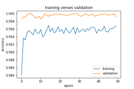
All three models performed well on validation data, they all resulted in more than 99% accuracy on validation data. Model3 used both the title and the text as input, the result is really close to 100%. For simplicity, I would recommend model1 or model2, but if we only focus on the performance result, the model3 is the best based on the output.
4. Model Evaluation
Test the model performance on unseen test data.
df_test = pd.read_csv("https://github.com/PhilChodrow/PIC16b/blob/master/datasets/fake_news_test.csv?raw=true")
df_test.head()
| Unnamed: 0 | title | text | fake | |
|---|---|---|---|---|
| 0 | 420 | CNN And MSNBC Destroy Trump, Black Out His Fa... | Donald Trump practically does something to cri... | 1 |
| 1 | 14902 | Exclusive: Kremlin tells companies to deliver ... | The Kremlin wants good news. The Russian lead... | 0 |
| 2 | 322 | Golden State Warriors Coach Just WRECKED Trum... | On Saturday, the man we re forced to call Pre... | 1 |
| 3 | 16108 | Putin opens monument to Stalin's victims, diss... | President Vladimir Putin inaugurated a monumen... | 0 |
| 4 | 10304 | BREAKING: DNC HACKER FIRED For Bank Fraud…Blam... | Apparently breaking the law and scamming the g... | 1 |
test = make_dataset(df_test)
test = test.batch(20)
model3.evaluate(test)
1123/1123 [==============================] - 4s 4ms/step - loss: 0.0257 - accuracy: 0.9946


[0.025698255747556686, 0.994565486907959]
The average accuracy for testing data is 99%, which is really good.
5. Embedding Visualization
weights = model3.get_layer('embedding2').get_weights()[0] # get the weights from the embedding layer
vocab = title_vectorize_layer.get_vocabulary()                # get the vocabulary from our data prep for later

from sklearn.decomposition import PCA
pca = PCA(n_components=2)
weights = pca.fit_transform(weights)

embedding_df = pd.DataFrame({
    'word' : vocab,
    'x0'   : weights[:,0],
    'x1'   : weights[:,1]
})
fig = px.scatter(embedding_df,
                 x = "x0",
                 y = "x1",
                 size = [2]*len(embedding_df),
                # size_max = 2,
                 hover_name = "word")

fig.show()
From the visualization, we can see a big cluster which means all those words could be found either in true news or fake news. The words near the center of the graph are the most common words in the news such as ‘services’, ‘everyone’, and ‘bad’ which may not be helpful for the model to determine whether the news is true or not. Also, in the graph, we can also see some outliers on the left or the right of the cluster such as ‘gop’, ‘gov’, ‘its’. Those outliers may indicate the news with these words is a trend to be fake or true news.